Summary
Transformers are complex. While textbooks are good at explaining theory, they often lack details. This document fills in the gap with low-cost experiments that clearly show the results when a transformer is pushed beyond its low frequency ratings.
![]() Estimated reading time: 10 minutes
Estimated reading time: 10 minutes
Introduction
Transformers are one of the most misunderstood basic components, second only to the inductor. This engineering brief outlines experiments you can conduct to improve your understanding. It emphasizes the low frequency response of the transformer leading to a better understanding of related questions:
-
Why are low frequency transformers larger than their high frequency counterparts?
-
Why did my 120 VAC transformer burn out when connected to 240 VAC?
-
What is core saturation and when is it first observed?
-
Why are audio transformers so large and heavy? This is especially important for vacuum tube guitar and audio amplifiers.
-
What are the bandwidth limitations of audio transformers?

Figure 1: Image of the small transformer with the Author’s Analog Discovery in the background.
Intended Audience
We assume familiarity with electronics such as the ability to use an oscilloscope and to read a Bode plot. You need to apply filters and op amps analytic concepts to the transformer (200-level topics). This is the perfect opportunity to revisit the transformer and overlay newly refined skills.
Tech Tip: This is out of sequence for electronics education, but maybe it shouldn’t be, as engineers don’t get transformers. Hint, hint, for your next job interview. The transformer is where theory meets the real world.
Review of the Voltage-to-Frequency (V/f) Ratio Equation
Before we describe the experiment, let’s take a quick look at the textbook transformer EMF equation (volts-per-turn-rule). This equation points to a maximum B field before the onset of saturation is described as:
B_{max} = \frac{V}{K \, N \, A \, f}
Where:
- B_{max} = Flux density (maximum)
- V = Applied RMS voltage
- K = Waveform constant of 4.44 for sinusoid signal derived from \frac{2 \pi}{\sqrt{2}}
- N = Number of turns
- A = Core area
- f = Frequency
We can simplify the base equation for a given transformer by rolling the K, N, and A terms into a single lumped constant applicable to a specific real-world transformer.
V = K \, N \, A \, f \, B_{max} \longrightarrow V = C \, f \, B_{max} \longrightarrow B_{max} = \frac{V}{C \, f}
Personally, I find this final form easier to understand and it certainly helps frame the experiments described in this document. Go ahead and write the relationship on a notecard.
Derivation of the Voltage-to-Frequency (V/f) Ratio Equation
The voltage to frequency equation is based on a first principal application of Faraday’s law:
e = N \frac{d\Phi}{dt}
We assume a sinusoidal voltage of:
e(t) = \sqrt{2}\,E_{RMS} \sin(\omega t)
Solving for flux lands us into integral calculus:
\Phi(t) = \frac{1}{N} \int e(t)\, dt
With substitution and calculus we derive the base equation:
B_{\text{max}} = \frac{V}{K \, N \, A \, f}
Required Components for the Transformer Experiment
Collect the components and test equipment for the experiments consisting of:
-
A small audio transformer such as the Triad Magnetics MET-31-T as shown in Figure 1. This transformer was chosen so that we can deliberately saturate the core at low frequencies.
-
A multifunction instrument capable of performing a spectrum sweep such as the Digilent Analog Discovery
-
Breadboard and common resistors.
-
Header pins to allow the Analog Discovery to be connected to the breadboard.
Tech Tip: Your lab may be equipped with a traditional signal generator and oscilloscope. That’s a wonderful situation. However, you will need to perform the frequency sweep manually and plot the results in a spreadsheet or on log paper.
Equipment Setup for the Transformer Frequency Sweep
The setup is shown in Figure 1 with the accompanying schematic in Figure 2. It includes:
-
Function generator driving the transformer
-
10 Ω shunt in series with the transformer used for current measurement
-
1 kΩ load resistor
-
Connect the oscilloscope to measure the voltage across R1 (input current representation) and R2 (output voltage).
In this example, the Analog Discovery operates as both function generator and oscilloscope.

Figure 2: Schematic for the transformer frequency sweep.
Experiments to Characterize the Transformer Response in Four Parts
The suggested experiments are subdivided into four sections. The first section establishes a baseline, while the later sections overload the transformer to reveal the low frequency response which supports the voltage-to-frequency (V/f) ratio equation.
Part 1: Initial Test Conducted at 1 KHz
Our first experiment is to verify that the system is working by feeding a 1 kHz signal to the transformer and observing the output voltage and input current. The target waveforms are shown in Figure 3. Observe:
- Waveform generator signal in red
- Output voltage (orange) is slightly attenuated
- Voltage and current (blue) are in phase
- Voltage and current are sinusoidal and relatively distortion free
Observations
This is an ideal situation with the transformer operating normally within its stated bandwidth.

Figure 3: Voltage and current waveforms for the transformer operating at 1 kHz.
Part 2: Frequency Sweep at Low Amplitude
The second experiment is to frequency sweep the transformer using the advanced features of the Digilent Analog Discovery. The results are shown in Figure 4. The transformer input amplitude is set to 50 mV.
-
The voltage (orange) is relatively flat dropping approximately 3 dB at 30 Hz.
-
The current (blue) increases significantly (18 dB) for the lowest frequencies.
Observations
This experiment demonstrates that the transformer’s frequency response is generally acceptable for small signals. It isn’t high fidelity (flat from 20 Hz to 20 kHz). However, it is certainly flat down to the lowest voice frequencies (300 Hz).
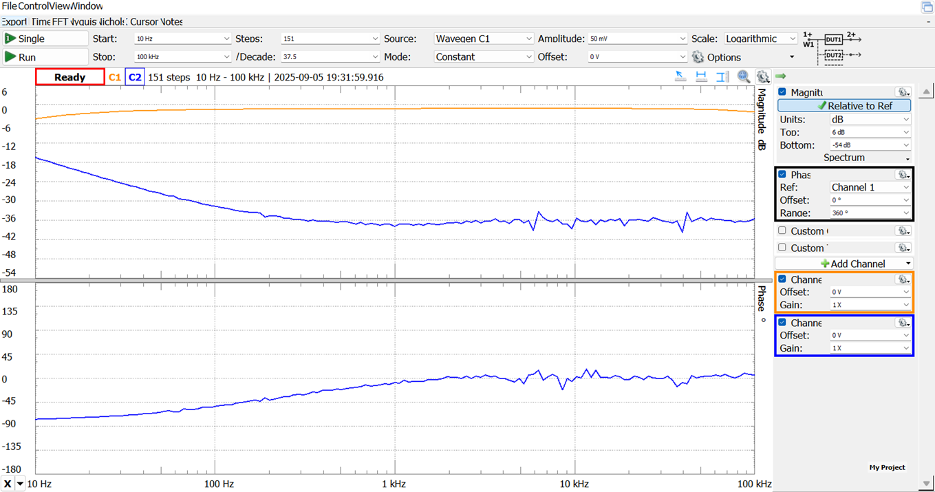
Figure 4: Signal sweep for the transformer at low signal level.
Part 3: Frequency Sweep at High Amplitude
This is the most important experiment in the series. Instead of feeding the transformer with a 50 mV signal we increase the amplitude to 5 V.
The resulting frequency sweep shown in Figure 5 stands in stark contrast with Figure 4.
-
The additional voltage causes the input current to increase by an astonishing 40 dB over midband current
-
The output voltage drops like a rock for frequencies less 200 Hz.
-
Despite this apparent deficiency, the transformer still operated perfectly within the datasheet specified low frequency limit of 300 Hz.
Observations
High voltages at low frequencies are associated with high currents in a transformer.
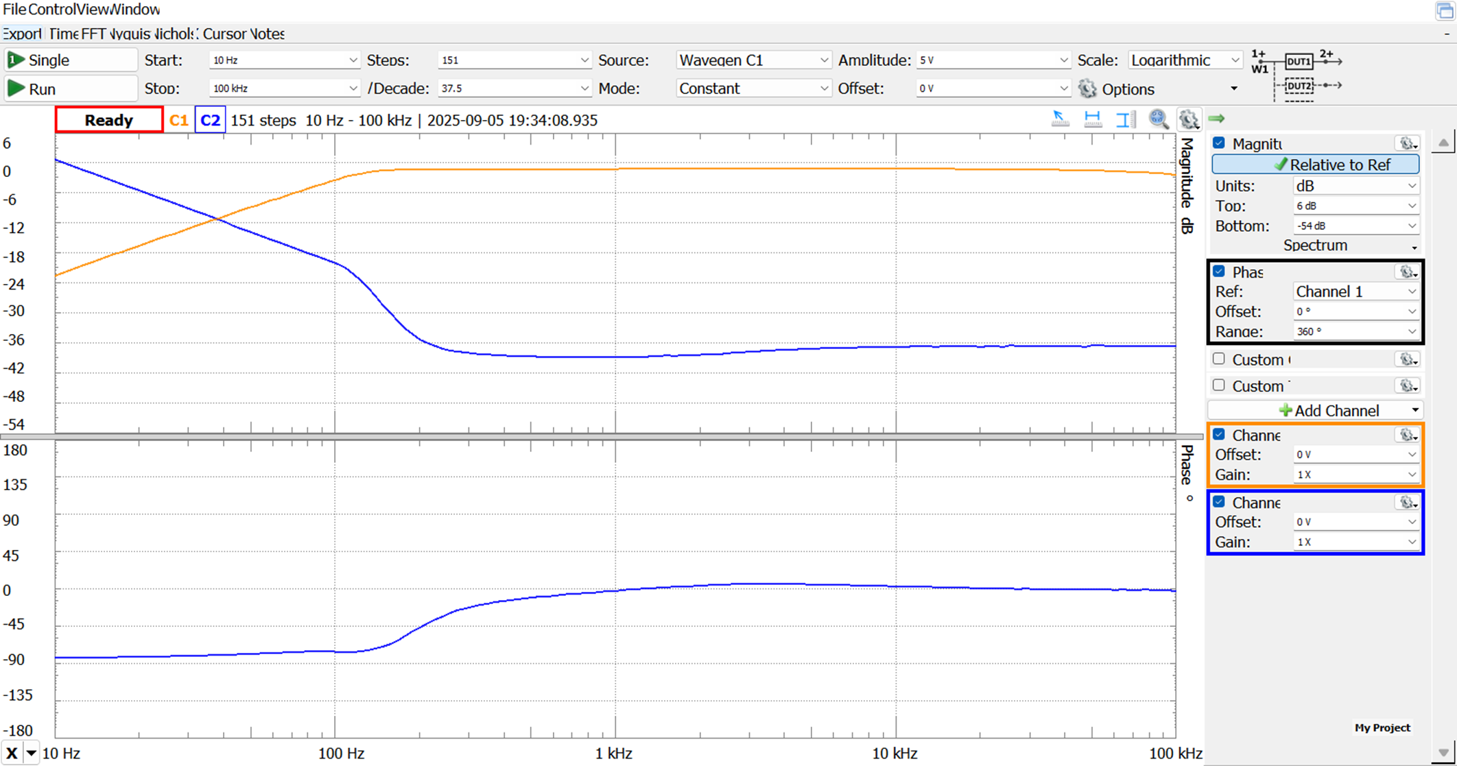
Figure 5: Signal sweep for the transformer operating at a high signal level.
Part 4: Close Inspection at Low Frequency High Amplitude
This experiment takes a closer look at the current resulting from high voltages at low frequencies. The settings are identical to those shown in Figure 3 except for the frequency which was changed from 1 kHz to 100 Hz. The resulting highly distorted current and voltage signals are shown in Figure 6.
Observations
We see significant spikes in the transformer’s input current. To fully understand the situation, we notice that the spikes occur when the input current is changing rapidly. This occurs at approximately 90 degrees relative to the input signal. Yet, you already knew that from the frequency sweep in Figure 5.

Figure 6: Voltage and current waveforms for the transformer operating at 100 Hz.
Interpreting the Results
TL;DR: The B-H curves are no longer linear at high voltages and low frequencies. This has nothing to do with the load.
From your electronics 101 class you know that the current in an inductor has a 90-degree shift (lagging) relative to the input voltage.
We can explain the current spike using a simple thought experiment.
Suppose we have two inductors. One has a high impedance while the other has a low impedance. If both are connected across a voltage source, the lower impedance inductor will have a higher current. We also note that the current in both cases lags the input voltage.
From Figure 4 we see that the current is relatively controlled for the 50 mV input signal. However, in Figure 5, the current increases significantly with a higher input voltage. Knowing what we know about inductors, we can reasonably assume that the transformer ran out of inductance at low frequencies. This is based on our observation of current spikes on the rising and falling edge of the input waveform (90-degree relationship between voltage and current).
As further evidence, consider Figure 7. Here we see the signal sweep when the load resistor is removed. We note that the low frequency input current is nearly identical between load and no load. This reinforces our assumption that we are running out of inductance. Stated another way the B-H curves are no longer linear, and it has nothing to do with the load. There is an implication that the primary winding will overheat with continued operation at high voltage at low frequencies.
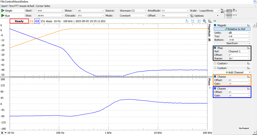
Figure 7: No load signal sweep for the transformer operating at a high signal level.
Refined Analysis
Technically, the core is saturating where saturation is dependent on the transformer construction and the applied frequency. We can relate this back to power transformers by recognizing that a transformer winding is designed for a given voltage at a specified (fixed) frequency.
For example, a cost sensitive power transformer winding is designed for 120 VAC at 60 Hz. Here the term cost sensitive implies that the designer has minimized the core material (iron). This same transformer would be unsuitable for 120 VAC and 50 Hz operation. The input voltage would cross the magnetization knee, saturating the core causing the same current spikes we see in Figure 6.
Suggested Follow-up Experiment Using a Spectrum Analyzer as a Saturation Meter
We can support the simplified equation by holding frequency constant and then increasing voltage until we reach the threshold of saturation. This may be an opportunity to use the spectrum analyzer to establish an experimental threshold. For example, we could define saturation as ratio between the fundamental and the 2nd or 3rd harmonic. This isn’t perfect but makes a reasonable saturation meter. We then move to other frequencies and see if the lumped C is constant for the transformer.
Parting Thoughts
The little audio transformer featured in this article, along with versatile test equipment, provides a bridge between practice and theory. The small size allows it to be overdriven (saturated) by the Analog Discovery revealing the low frequency characteristics.
Give it a try and let us know if your students were successful.
Best wishes,
APDahlen
Related Articles by this Author
If you enjoyed this article, you may also find these related articles helpful:
- How to select resistor pairs for op amp and voltage divider applications
- What is the purpose of the emitter bypass capacitor in the Common Emitter (CE) amplifier?
- Wien Bridge Oscillator Construction and Performance
- How to Interface a Microcontroller with a Relay Using a MOSFET
About This Author
Aaron Dahlen, LCDR USCG (Ret.), serves as an application engineer at DigiKey. He has a unique electronics and automation foundation built over a 27-year military career as a technician and engineer which was further enhanced by 12 years of teaching (interwoven). With an MSEE degree from Minnesota State University, Mankato, Dahlen has taught in an ABET-accredited EE program, served as the program coordinator for an EET program, and taught component-level repair to military electronics technicians.
Dahlen has returned to his Northern Minnesota home, completing a decades-long journey that began as a search for capacitors. Read his story here.