← Previous Analog Bits - Wheatstone Bridge Input and Output Resistance
Analog Combinator Circuit for Load Cells - Next Analog Bits →
In the previous article the following was shown for a perfectly balanced symmetrically complimentary load cell.


Where Rs is the span compensation resistance, Ro is the at rest strain gauge resistance (equal to the rated output resistance when zero force is applied), and the added/subtracted resistance due to applied force is Rf .
Note that it is assumed anything that may be connected to the signal output is high enough in impedance to have negligible impact.
Download A Free Version of Mathcad
Download LTspice for Free
Calculating Rf Using Symmetry
The desire is to consider a real load cell that provides ratings for its:
- Output resistance at zero load ( Ro ), also equal to the at rest resistance of each strain gauge.
- Span compensation resistors ( Rs ).
- Load range ( lbfmax ), operating force, e.g. a 100 lbf cell.
- Full scale output span ( Vfsos ), signal volts per volt of excitation at maximum load.
As will be seen, this means the only unknown that needs to be solved for to create a proper load cell model is Rf .
It’s convenient to relabel some elements in the above circuit representation, and to consider the negative excitation lead the circuit ground.

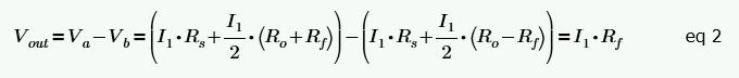
The excitation voltage is now Vin , and the positive and negative output signal voltages are Va and Vb respectively, which would make the output voltage, Vout = Va - Vb . In this case for a perfectly balanced symmetrically complimentary load cell, it’s possible to exploit the symmetry of the circuit to make the algebra much simpler. Due to Kirchhoff’s Current Law and the symmetry of the four bridge strain gauge resistances, the three unknown currents have the following relationships.

Since Vout = Va - Vb , applying Kirchhoff’s Voltage Law to find Va and Vb and substituting them in along with eq 1 for I2 and I3 yields the following.
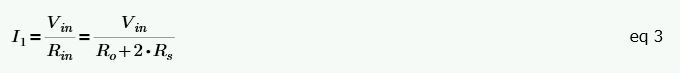
Since the input resistance is already known, I1 can be written easily via Ohm’s law.
Substituting eq 3 in to eq 2 and solving for Rf yields the following.

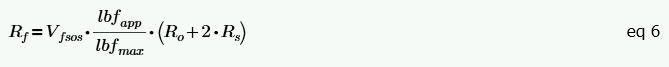
Vout/Vin is just the transfer ratio, and the datasheet effectively provides this via the full scale output span, Vfsos , and maximum load rating, lbfmax . Vfsos must simply be scaled linearly by the ratio of the actual applied force, lbfapp , to lbfmax .

Substituting eq 5 in to eq 4 then yields the following.
If you would like the Mathcad file for the above, you can download it here:Load_Cell_Symmetry.mcdx (111.2 KB)
Another Interesting Result of the Symmetry
Eq 6 is really what we are after for our simulation model, but I think it’s worth taking a minute to appreciate another aspect that results from the perfectly balanced symmetrically complimentary nature of a load cell like this. Consider that from eq 4 , Rf is in fact just the transfer ratio multiplied by the input resistance. If this equation is rearranged, it can be looked at in a different way.
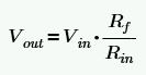
Arranged this way, and considering that the various Rf added/subtracted values in the circuit are in fact a part of Rin (they cancel each other out, but they are a part of it), it can be looked at as a simple voltage division equation where the output voltage is simply the portion of the input voltage that results across a single Rf .
This left me pondering why that is, but after considering that the actual change in resistance in each leg of the Wheatstone bridge is 2 ***** Rf , and from the input resistance perspective the two legs are in parallel with each other, (2Rf) || (2Rf) = Rf , the relationship became more apparent.
This same relationship can be seen in a different way as well. In eq 2 it was effectively written that ![]() , and of course
, and of course  .
.
An extremely clever person could have written the equation for Rf from inspection and avoided any calculations, but unfortunately that extremely clever person isn’t me.
Other Methods of Calculation
There are of course other ways to arrive at the same equation for Rf . If you are foolish like me and set in your ways you might start with Nodal Analysis. This made perfect sense at the time since the initial goal was to find Va and Vb , two node voltages. I wouldn’t recommend this approach, but if you are curious how awful the algebra becomes, you can see it in the Mathcad file here: Load_Cell_Nodal.mcdx (149.6 KB)
If you are a little more clever you would use Mesh Analysis, after all, there are four unknown node voltages but only two unknown mesh currents. The algebra is less awful this way, but still not nearly as simple as the symmetry approach used above. Mathcad file here: Load_Cell_Mesh.mcdx (131.9 KB)
The Unamplified Load Cell Model
The unamplified load cell model below created in LTspice can be download here:UnamplifiedLoadCellModel.asc (1.4 KB)
The parameters the user must set are:
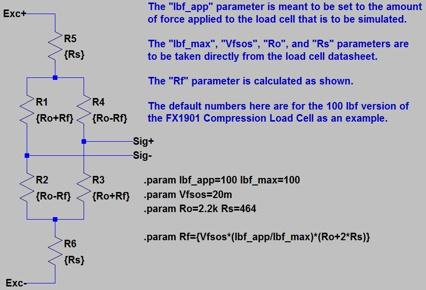
- lbf_app is meant to be set (or swept) to the amount of force applied to the load cell for the simulation.
- lbf_max is maximum rated operating force of the cell (e.g. a 100 lbf cell).
- Vfsos is the full scale output span (signal volts per volt of excitation at maximum load).
- Ro is the output resistance at zero load, which also equal to the at rest resistance of each strain gauge.
- Rs is the value of the span compensation resistors if any (can be set to zero if there are none).
The default numbers are for the Measurement Specialties FX1901-0001-0100-L compression load cell at maximum load.
Modeling the load cell this way keeps the simulation true to life regarding how it will behave as both an electrical load to its connected excitation, and for how it will behave differently due to any connected electrical load at its signal outputs. The electro-mechanical behavior as lbf_app is adjusted is “ideal” since there is no non-linearity in the model, nor accounting of any changes due to temperature or secondary mechanical effects such as drift, creep, or hysteresis. The applied force can be positive or negative for load cell types that can be put under compression or extension, but of course the user should keep the values within the rated range of the load cell being simulated.
Testing The Unamplified Load Cell Model
The simple test of the unamplified load cell model in LTspice can be downloaded here: UnamplifiedLoadCellModel_Test.asc (1.3 KB)

The excitation voltage is a simple 5V source and the signal output is unloaded, as shown. The ideal expected behavior under these conditions is shown in the plot output where the x-axis is lbf_app .
Why Not Just Use a Voltage Dependent Voltage Source?
I imagine a lot of people that want to simulate a load cell first start with the idea of a simple voltage dependent voltage source (I certainly did). If a crude approximation is good enough then this might be just fine, but there are drawbacks to this. Most of the drawbacks can be compensated for by making the model a little more complex, but not all.
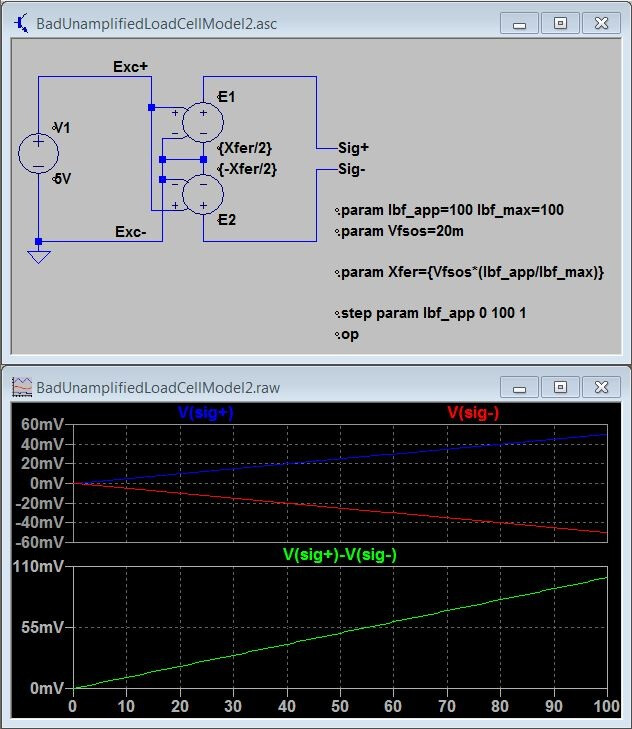
If we consider just a single voltage dependent voltage source, the first major drawback is that it will behave as a single ended output source instead of a differential one.

But hey, we could always be a little more clever and use two appropriately connected and adjusted voltage dependent voltage sources to get a differential output.
Of course, that is differential around GND , and technically it’s supposed to be differential around half the excitation voltage, so we might want to fix that with a little more complication by either adding another voltage dependent voltage source to provide the appropriate DC offset, or to otherwise modify the existing two transfer equations to include it.
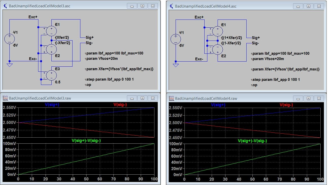
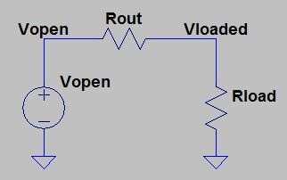
There, now that’s looking better, of course we may also want whatever the source of the excitation voltage in our simulation is to see the load that would be presented by the load cell itself (more difficult to also consider any load that would be connected to the signal outputs). It would be difficult to accomplish this well, but we do have an equation for input resistance of a load cell, and we could add a simple resistor along with the necessary parameters to approximate this poorly (probably good enough, right?).

Of course, now that we have our overly simplified approximation of input resistance, we best do the same for the output resistance (more difficult to also consider any source impedance from the actual excitation source). Again, we do have an equation for output resistance of a load cell, and we could add a simple resistor (actually two to keep it differentially balanced) along with the necessary additional parameters to approximate this poorly as well.

Okay, so now we have a model that isn’t too horrible. It will, with a sufficiently high output impedance signal load, present something close to the expected input impedance to the excitation source. Also, it will, with a sufficiently low excitation source output impedance, present something close to the expected output impedance to the connected signal load.
Oh sure, the Input and Output Resistance values don’t automatically adjust (as they would in reality) for whatever is connected to the excitation and signal leads, and sure, there is a false (i.e. doesn’t exist in reality) buffer between the excitation source and the signal output via the dependent sources, and sure, in addition to being less true to life this model is also more complicated to set up and less intuitive to understand, but… but… wait where was I going with this argument?
In summary, this just isn’t nearly as good a way to model a load cell as what was previously provided, for all the reasons listed in the last paragraph.
Unamplified Load Cell Models Comparison
For a simple demonstration of the deficiencies in the voltage dependent voltage sources model, consider the following example of both unamplified load cell models modestly loaded at their signal outputs with 100k resistors to ground and a 100k differential resistance.

There are subtle differences in results. While the differential output voltage is hardly different at all (it is slightly), the output signal voltages relative to ground are shifted about 15mV further down from their ideal (infinite load resistance) values in the original model, as they should be due to the additional signal loading. This is because the voltage dependent voltage sources model sources output current from the dependent sources instead of the excitation voltage as it would in reality. For the same reason, the voltage dependent voltage sources model excitation voltage’s output current is about 25uA less, and doesn’t show the same mild 30nA bend downward as the applied force increases. Your application may not care about 15mV, 25uA, or 40nA (it probably doesn’t), but what if your application excitation source and/or signal load had more of an impact? Why wouldn’t you want to use a model that is more likely to help you catch problems you may not have noticed or thought of, and that’s easier for you to understand too?
If you are the type who likes solving problems just for the sake of solving problems, you could have a little fun trying to find ways to improve the voltage dependent voltage sources model and make it more true to life, and if you would like to do so be by guest, here is the LTspice test for it from above for your convenience:
UnamplifiedLoadCellModel2_Test.asc (1.6 KB)
Just remember that the original resistor only model solved all these problems already without any additional complication.
The Amplified Load Cell Model
The amplified load cell model below created in LTspice can be download here: AmplifiedLoadCellModel.asc (2.7 KB)

The parameters the user must set are:
- lbf_app is meant to be set (or swept) to the amount of force applied to the load cell for the simulation.
- lbf_max is maximum rated operating force of the cell (e.g. a 100 lbf cell).
- Vfsos is the full scale output span (signal volts per volt of excitation at maximum load) of the unamplified Wheatstone bridge.
- Vexc is the datasheet specified operating voltage supply at which Vspan and Vo are specified.
- Vspan is the datasheet specified amplified output voltage swing when Vexc is the operating voltage supply.
- Vo is the amplified zero force output voltage (can be set to zero if zero) when Vexc is the operating voltage supply.
- Ro is the Wheatstone bridge output resistance at zero load, which also equals to the at rest resistance of each strain gauge.
- Rs is the value of the span compensation resistors if any (can be set to zero if there are none).
- Rout is the output resistance at the amplified output (can be determined through testing and calculation if not specified, or set to zero).
- Iq is the quiescent current of the amplifier circuit (can be determined through testing and calculation if not specified, or set to zero).
The default numbers are for the Measurement Specialties FC2231-0000-0100-L compression load cell (with the exception of Rout and Iq ) at maximum load.
Modeling the load cell this way is essentially a work around for the fact that most load cell manufacturers provide (seemingly intentionally) very little information in their datasheets about the details of their amplification circuits (let alone an actual SPICE model for them). The electro-mechanical behavior as lbf_app is adjusted is “ideal” since there is no non-linearity in the model, nor accounting of any changes due to temperature or secondary mechanical effects such as drift, creep, or hysteresis. The electrical behavior of the amplification is “ideal” as well since there is similarly no non-linearity in the model, nor accounting for any changes due to temperature or other non-ideal electrical behaviors inherent to any actual amplifier circuit. The applied force can be positive or negative for load cell types that can be put under compression or extension, but of course the user should keep the values within the rated range of the load cell being simulated.
It is possible for this model, since its output is based on a dependent voltage source, to swing above the Exc+ voltage or below the Exc- voltage if out of range and/or nonsense numbers are put in to the parameters, but of course this wouldn’t be possible in reality. It’s also possible to connect any arbitrary voltage across the excitation leads and get output, even though the actual amplification circuit would require some minimum voltage to operate and at some maximum voltage would cease to operate or become damaged. In other words, it’s important the parameters are realistic or it’s nonsense in and nonsense out.
Testing The Amplified Load Cell Model
The simple test of the unamplified load cell model in LTspice can be downloaded here: AmplifiedLoadCellModel_Test.asc (2.3 KB)

The excitation voltage is a simple 3.3V source. Notice that the parameters for Vexc , Vspan , and Vo didn’t need to be adjusted from their datasheet given 5V numbers at all since these parameters are ratio-metric to the supply and the model automatically adjusts. Also notice that I’ve intentionally put somewhat large arbitrary values in for Rout (100 Ohm) and Iq (1 mA) to more clearly demonstrate the change in model behavior as the output is loaded.
The ideal expected behavior under these conditions is shown in the plot outputs where the x-axis is lbf_app . In the left plot for the open load circuit the excitation source sees a static 2.1mA load as the output voltage swings from exactly 10% to 90% of the excitation voltage. In the right plot for the 1k Ohm output load the excitation source sees a linearly increasing load from 2.4 mA to 4.8 mA as the output voltage swings from 300 mV to 2.7V as would be expected with the additional voltage drop across Rout .
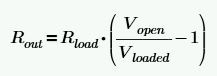
Optional: How to Test and Calculate Rout and Iq
For an amplified load cell, resistance of the Vout wire itself (which of course varies with temperature) may actually be the dominant component of Rout , although it’s unlikely to matter much unless you have very long thin wires. For example, 30 feet of 32 gauge wire would be about 5 Ohms at room temperature, but the 3 feet of 22 gauge wire you are more likely to encounter on an off-the-shelf load cell would only be one twentieth of an Ohm. But, there could be other unknown dominant factors, and if you need to quantify Rout the process is simple enough. Go ahead and hook up your load cell to your excitation power supply, and then ideally apply the maximum rated force to it for maximum voltage output (more voltage for more headroom to measure). Take a Vout measurement with an open circuit output, and then take another measurement while loading the output (the larger the current draw the better, again for headroom, but of course don’t overload your load cell output). After that it’s just working a simple two resistor voltage divider backward to find the missing resistance.
Iq is even easier as long as you have an accurate enough low current meter. With an open circuit output at Vout , measure the current draw from your excitation voltage power supply. Now do some simple Ohm’s Law math to subtract out the portion that you know is flowing through the Wheatstone Bridge circuit (the excitation voltage divided by the Wheatstone bridge input resistance), and what’s left is Iq .
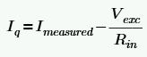
Recall that the equation for the Wheatstone bridge input resistance, Rin , if it isn’t directly specified in your load cell datasheet, is at the top of this page. Also, an explanation of it can be found in the previous Analog Bits article.
The Amplified Load Cell Model in a Perfect World
If the world were perfect, I would recommend you use the model given to you by your load cell manufacturer (which they almost certainly won’t provide), or that you ask them to provide you the schematic and BOM of their amplification circuit so you can build your own (which they are very unlikely to provide), or that you, me, anyone else tear apart a sacrificial load cell and reverse engineer the entire thing (which none of us will unless we work for a competitor of that load cell manufacturer because it’s just not worth the trouble otherwise). So, like most electronics manufacturers, they have managed to stay the course and conceal valuable information from their customers under the erroneous presumption that their competitors won’t “figure it out” anyway because they have a large financial incentive to do so. But I digress.
Since I can’t actually make the things above happen in reality, I’ll have to play pretend a little to give you an example of what would be an even better model. Let’s pretend I did manage to get all the internal details for some amplified load cell. Well, then I would model it as exactly as I could, like this (again my model is very made up, the E1 and E2 dependent sources for offset should be a dead giveaway)…

In this case, my imaginary load cell uses the LTC2053 instrumentation amplifier set for a gain of 40, which I picked because it clearly demonstrates majorly important behaviors that are lost in the entirely dependent sources model. The major behaviors in question are that the LTC2053 has a switched input that samples via a capacitor the input signal voltage from the Wheatstone bridge every 333us (by default), its output voltage is actually high at startup, and then there is a relatively long amount of output settling time that gets worse the closer the output will be to the positive rail. In fact, because of the switched input nature a DC operating point simulation becomes meaningless (LTspice even warns you if you try), so the simulation has to be done as a transient sim with a long enough time period to see the output settle as lbf_app is swept.
Now I realize that this load cell is imaginary, but if any real load cell had similar behavior that’s necessarily lost in the previously provided model based entirely on dependent sources, the user of said load cell would have to realize this and potentially understand all the behavior lost in the more “ideal” model being utilized. Unfortunately, the world isn’t perfect, and neither is any model.
Why Not Just Use a Single Voltage Source?
Oh come on, now you’re just being lazy, aren’t you?

I mean, take a little pride in your work. Yes, you can do this for the most absolutely quick and dirty model possible, but it certainly isn’t going to dynamically adjust for whatever you connect it to. There are no excitation connections for crying out loud! Basically, don’t do this for most of the same reasons that were covered for not using a single voltage dependent voltage source for an Unamplified Load Cell.
Links to Additional Load Cell Information
Rice Lake Load Cell Handbook - A great deal of good information here regarding load cell theory, types, construction, selection, measurement/conversion, troubleshooting, and terminology.
SparkFun’s Getting Started with Load Cells - Some very nice visuals here that can help you understand how “perfectly balanced and symmetrically complimentary” works in practice for load cells.
Load Cell Error Theory - Explanations for several sources of error in real load cells.